Lesson 17.1: Characteristics of Populations

 

Lesson Objectives

 

Recognize that human concern about overpopulation dates to ancient Greek times.

Explain that Cornucopians believe that technology will solve population problems.

Connect the study of the biology of natural populations to better understand human population issues.

Define a biological population.

Give reasons why biologists study populations.

Compare the importance of population size to that of population density.

Explain how conservation biologists use Minimum Viable Population (MVP) and Pop- ulation Viability Analysis (PVA).

Explain how patchy habitats influence the distribution of individuals within a popula- tion.

Define and explain the reasons for three patterns of dispersion within populations.

Describe how population pyramids show the age and sex structures of populations.

Interpret population pyramids to indicate populations’ birth and death rates and life expectancy.

Analyze the effect of age at maturity on population size.

Explain the structure and meaning of a generalized survivorship curve.

Compare and contrast the three basic types of survivorship curves.

Introduction

“Solving the population problem is not going to solve the problems of racism… of sexism… of religious intolerance… of war… of gross economic inequality—But if you don’t solve the population problem, you’re not going to solve any of those problems. Whatever problem you’re interested in, you’re not going to solve it unless you also solve the population problem. Whatever your cause, it’s a lost cause without population control.” –Paul Ehrlich, 1996

(From Paul Ehrlich and the Population Bomb, PBS video produced by Canadian biologist Dr. David Suzuki, April 26, 1996.)

What exactly is the population problem? How can it be solved?

 

 

Humans have shown concern for overpopulation since the Ancient Greeks built outposts for their expanding citizenship and delayed age of marriage for men to 30. In 1798, Thomas Malthus predicted that the human population would outgrow its food supply by the middle of the 19th century. That time arrived without a Malthusian crisis, but Charles Darwin nevertheless embraced Malthus’ ideas and made them the foundation of his own theory of evolution by natural selection. In a 1968 essay, The Tragedy of the Commons, Garrett Hardin exhorted humans to “relinquish their freedom to breed,” arguing in the journal, Science, that “the population problem has no technical solution,” but “requires a fundamental extension in morality.” In 1979, the government of China instituted a “birth planning” policy, charging fines or “economic compensation fees” for families with more than one child. Others have opposing views, however. Julian Simon, professor of Business Administration and Senior Fellow at the Cato Institute, argued that The Ultimate Resource is population, because people and markets find solutions to any problems presented by overpopulation. A group known as cornucopians continues to promote the view that more is better.

Would you support a law forbidding you to marry until a certain age? Do you know how such a law would affect population growth? Would you limit the size of all families to one child (Figure 17.1)? Do you believe families should welcome as many children as possible? Should these decisions be regulated by law, or by individual choice? Clearly, the “population problem” reaches beyond biology to economics, law, morality, and religion. Although the latter subjects are beyond the scope of this text, the study of population biology can shed some light on human population issues. Let’s look at what biologists have learned about natural populations. Later, we will look more closely at human populations, and compare them to populations in nature.

 

 

Measuring Populations

In biology, a population is a group of organisms of a single species living within a certain area. Ecologists study populations because they directly share a common gene pool. Unlike the species as a whole, members of a population form an interbreeding unit. Natural selection

 

 

Figure 17.1: The Chinese government mandates population control by charging “economic compensation fees” for families with more than one child. (22)

 

acts on individuals within populations, so the gene pool reflects the interaction between a population and its environment.

Biologists study populations to determine their health or stability, asking questions such as:

 

Is a certain population of endangered grizzly bears growing, stable, or declining?

Is an introduced species such as the zebra mussel or purple loosestrife growing in numbers?

Are native populations declining because of an introduced species?

What factors affect the growth, stability, or decline of a threatened population?

 

The first step in characterizing the health of a population is measuring its size. If you are studying the population of purple loosestrife plants on your block , you can probably count each individual to obtain an accurate measure of the population’s size. However, measuring the population of loosestrife plants in your county would require sampling techniques, such as counting the plants in several randomly chosen small plots and then multiplying the average by the total area of your county. For secretive, highly mobile, or rare species, traps, motion- detecting cameras, or signs such as nests, burrows, tracks, or droppings allow estimates of population size.

 

 

Figure 17.2: Purple loosestrife plant populations show patchiness due to uneven distribution of their wetland habitats, and clumped dispersion, due to local variation in soils. (29)

 

Two problems with absolute size lead ecologists to describe populations in other terms. First, because your county may not be the same size as others, the total number of individuals is less meaningful than the population density of individuals – the number of individuals per unit area or volume. Ecologists use population densities more often for comparisons over space or time, although total number is still important for threatened or endangered species.

Concern about threatened and endangered species has led conservationists to attempt to define minimal viable population size for some species. A species’ MVP is the smallest

number of individuals which can exist without extinction due to random catastrophic vari- ations in environmental (temperature, rainfall), reproduction (birth rates or age-sex struc- ture), or genetic diversity. In 1978, Mark Shaffer incorporated an estimate for grizzly bear MPV into the first Population Viability Analysis (PVA), a model of interaction be- tween a species and the resources on which it depends. PVAs are species-specific, and require a great deal of field data for accurate computer modeling of population dynamics. PVAs can predict the probability of extinction, focus conservation efforts, and guide plans for sustainable management.

 

Patterns in Populations I: in Space (or Patterns in Space)

A second problem in measuring population size relates to the distribution of individuals within the population’s boundaries. If your county has extensive wetlands in the southern half, but very few in the north, a countywide population density estimate of purple looses- trife, which grows primarily in shallow freshwater pond edges, marshes, and fens, would be misleading (Figure 17.2). Patchy habitat – scattered suitable areas within population boundaries – inevitably leads to a patchy distribution of individuals within a population. On a smaller scale, plants within even a single wetland area may be clumped or clustered (grouped), due to soil conditions or gathering for reproduction. The characteristic pattern of spacing of individuals within a population is dispersion (Figure 17.3). Clumped dispersion is most common, but species that compete intensely, such as cactus for water in a desert, show uniform, or evenly spaced, dispersion.

 

 

Figure 17.3: Populations of cacti in the desert, such as this group of cholla, show uniform, or even, dispersion due to fierce competition for water. The diagrams to the right show nearly uniform (top), random (middle), and clumped (bottom) dispersion patterns. (31)

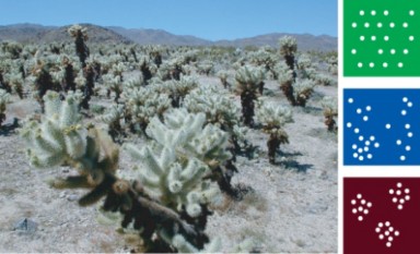
Other species, whose individuals do not interact strongly, show a random, or unpredictable, distribution. Useful measures of population density must take into account both patchiness of habitat and dispersion of individual organisms within the population’s boundaries.

 

Age-Sex Structure of a Population

 

 

Figure 17.4: Grizzly bear populations include adults up to 25 or 30 years old, capable of reproducing, and young immature bears under 6 years old. Healthy populations include roughly equal proportions of each age group. (6)

Density and dispersion describe a population’s size, but size is not everything. Consider three populations of endangered grizzly bears, each containing one individual per 20 km2, and a total of 100 individuals in 2,000 km2. These populations are “equal” with respect to size. One population, however, has 50 immature (non-reproducing young) bears and 50 adult bears able to reproduce. A second population has the same number of immature and adult bears, but of the 50 adults, 45 are male. The third population has 30 immature bears and 70 bears of reproductive age. Which population is healthiest (Figure 17.4)?

The answer is not simple, but age and sex differences between populations are significant indicators of health. Biologists concerned about a population’s future study age and sex within the population and then graph the results to show the age-sex structure as a population pyramid, although the result does not always resemble a pyramid. The X-axis in this double bar graph indicates percentage of the population, with males to the left and females to the right. The Y-axis indicates age groups from birth to old age.

The population in the generalized example (Figure 17.5) contains a large proportion of young individuals, suggesting a relatively high birth rate (number of births per individ- ual within the population per unit time). The bars narrow at each age interval, showing that a significant number of individuals die at every age. This relatively high death rate (number of deaths per individual within the population per unit time) indicates a short life

Figure 17.5: A generalized age-sex structure or population pyramid shows the proportion of males and females (X-axis) at each age level (Y-axis). This example shows a slightly higher proportion of females compared to males, and a much higher proportion of young individuals compared to old. (36)

 

 

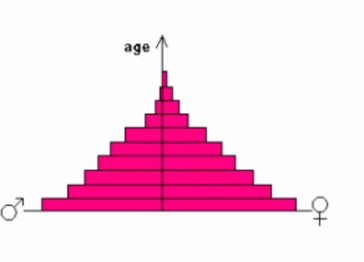
expectancy, or average survival time for an individual. Note the slightly greater propor- tion of females compared to males at each age level. Careful study could determine whether the cause for this imbalance is the ratio of female to male births, or higher death rates for males throughout a shorter lifespan. You will learn in a later lesson that this pattern is characteristic of human populations in less developed countries.

 

 

Figure 17.6: Age structures can reveal a population’s health. Type I, with most individuals below reproductive age, often indicates a growing population. Type II, with roughly equal proportions of the population at each age level, indicates a stable population. Type III, with more individuals at (or above!) reproductive age than young, describes a declining population. (38)

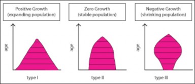
A population’s age structure may reveal its health (Figure 17.6). A growing population

(Type I) usually has more young individuals than adults at beyond reproductive age. A stable population (Type II) often has roughly equal numbers of young members and adults. A declining population shows more adults and fewer young (Type III). Sex structure may also affect the health of a population. Sex determination in sea turtles, for example, is temperature-dependent; lower egg incubation temperatures produce males, while tempera- tures as little as 1-2oC higher produce females (Figure 17.7). Some biologists predict that climate change may result in sea turtle sex structure shifts toward females, which could further endanger already threatened species. Continued monitoring of age-sex structures among sea turtles might be able to detect such changes before they become irreversible.

 

 

Figure 17.7: The sex of a sea turtle is determined by the temperature at which it develops – males in cooler temperatures, and females in temperatures as little as 1-2oC warmer. Climate change may threaten natural sex ratios. Such changes would be reflected in changing age-sex structure pyramids. (5)

 

Although it is not shown in population pyramids, an important factor affecting population size is the age at which individuals become able to reproduce (Table 17.1). Recall that age at maturity (when reproduction becomes possible) was the factor that even ancient Greeks recognized could affect population growth, when they prohibited marriage for males under the age of 30. We will return to this relationship in a later lesson, but for now, try to grasp it intuitively: if a person delays reproduction until age 30 and then has one child each year for two years, his or her fertility is 2. A person who has two children, one each year, beginning at age 20 also has a fertility of 2. Assume that these four children are born in the same two-year period, and that each offspring reproduces two children at the same age as his/her parent did. Sixty years after the initial four childbirths, the “delayed reproduction” individual will have 2 X 2 X 2 = 8 descendants. However, the early reproducing family will have 2 X 2 X 2 X 2 = 16 offspring – double the population increase of the first family. Do you think this could this be one way to slow human population growth?

 

Table 17.1: Number of Offspring Produced Over Time

Age at First Reproduc- tion

Initial Re- production

20 years later

30 years later

40 years later

60 years later

20 years Generation

1: 2 off- spring

30 years Generation

1: 2 off- spring

Generation 2: 4 off- spring

 

Generation 2: 4 off- spring

Generation 3: 8 off- spring

Generation 4: 16

Generation 3: 8

 

Patterns in Populations Through Time

 

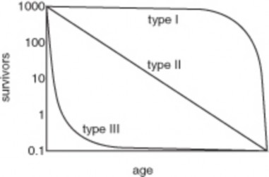
The characteristics of populations introduced above – birth rate, death rate, and life ex- pectancy – interact to form several basic strategies for survival. Insurance companies began investigations into life expectancies for various groups of people – males vs. females, for example – and compiled the data in life tables. Biologists plot these patterns through time in survivorship curves, which graph the number of all individuals still living (in powers of ten, on the Y-axis) for each age (on the X-axis). The three basic types of survivorship curves are illustrated in Figure 17.8.

Species showing a Type I pattern have the highest survival rates, with most individuals living to old age. Many large animals, including humans, show this “late loss” pattern of survivorship; few offspring, high levels of parental care, and low “infant” death rates characterize Type I species. As we will see in a later lesson, human populations in rich countries fit this pattern more closely than do those in undeveloped countries.

Species with Type III survivorship patterns experience high death rates among offspring; relatively few survive to old age. Most plants and invertebrates and many fish show this “early loss” pattern. Parents invest most of the reproductive energy in high numbers of offspring to offset the high death rates, and little or no energy remains for parental care.

Species showing intermediate, Type II survivorship curves experience uniform death rates throughout their lives. Some birds and many asexual species show this “constant loss” pattern.

We’ll look at these strategies more closely in the next lesson as we study how populations grow and change: population dynamics.

 

Figure 17.8: Survivorship curves correlate with strategies species use to adapt to various environments. Large organisms in relatively stable environments have few offspring but high levels of parental care; most individuals survive to old age (Type I). Smaller organisms in less stable environments produce many offspring but provide little parental care, and few survive to old age (Type III). Type II species show intermediate characteristics in response to a death rate which remains constant throughout life. (33)

Lesson Summary

Historic concern with overpopulation includes ancient Greek delay of marriage, Malthus’ predictions of a resource crisis, and Darwin’s use of exponential growth in his theory of natural selection.

A group lead by Julian Simon, cornucopians, believes that more people are better, because technology and innovation will solve population problems.

The study of the biology of natural populations can shed light on human population issues.

 

In biology, a population is a group of organisms of a single species living within a certain area.

Population size, the total number of individuals, is important for understanding endan- gered or threatened species, but population density is often more useful for comparing populations across time or space.

Minimum Viable Population (MVP) and Population Viability Analysis (PVA) use extensive field data to predict best management practices for a particular species in conservation biology.

 

Double bar graph population pyramids show proportions of males and females within age groups.

Population pyramids which have wide bases indicate high birth rates and probable population growth, and decreases from one age group to the next indicate death rates and (overall) life expectancy. Populations with narrow bases indicate low birth rates and shrinking populations, and those with bases roughly equal to peaks indicate stable populations and/or low death rates.

Delaying reproduction or increasing age to sexual maturity can decrease population growth rate, even if fertility levels remain the same.

 

Patchy habitat distribution results in patchy distribution of a population throughout its boundaries.

Dispersion of a population within its boundaries depends on intraspecies competition or cooperation.

 

 

Clumped distribution indicates social relationships or recent reproduction without dis- persal.

Uniform distribution reveals competition among individuals for a limited resource.

Random distribution suggests little interaction among individuals.

Survivorship curves show the number of individuals which survive (on a power-of-ten scale) at each age level.

 

 

Review Questions

 

Further Reading / Supplemental Links

Large animals, which provide few offspring with high levels of parental care, experience low death rates and long average life expectancy – a Type I pattern. This pattern is typical for humans in rich/developed countries.

Among plants and many invertebrates which have many offspring but little or no parental care, offspring have high death rates and relatively low average life expectancy

– a Type III pattern.

Some birds and many asexually reproducing species have constant death rates through- out life and intermediate average life expectancy – a Type II pattern.

Compare the cornucopian perspective on human population growth to the Malthus’ (sometimes called the Neo-Malthusian) view.

(If false, restate to make true.) Human concern about overpopulation is a recent phenomenon.

Define a biological population.

Define and compare the importance of population size vs. population density.

Explain how conservation biologists use Minimum Viable Population (MVP) and Pop- ulation Viability Analysis (PVA).

How does patchy distribution differ from dispersion?

What types of information do population pyramids show? What kinds of inferences can you make using variations in population pyramid shape?

How does delaying reproduction affect population size, even if fertility remains con- stant?

Describe the three types of survivorship curves and the reproductive strategies they illustrate.

Apply what you have learned so far about population biology to your current under- standing of human populations. Note: we will explore human populations in detail in a future lesson, so accept that your current understanding may be incomplete!

http://www.estrellamountain.edu/faculty/farabee/biobk/BioBookpopecol.html

http://www.geography.learnontheinternet.co.uk/topics/popn1.html

http://www.census.gov/ipc/www/idb/faq.html

http://www.biologicaldiversity.org/swcbd/species/orca/pva.pdf

http://nationalzoo.si.edu/ConservationAndScience/EndangeredSpecies/PopViability/ default.cfm

 

Vocabulary

age at maturity The age at which individuals (sometimes considered only for females) become able to reproduce.

 

age-sex structure A graphical depiction of proportions of males and females across all age groups within a population; also depicted as a population pyramid.

 

birth rate (b) The number of births within a population or subgroup per unit time; in human demography, the number of childbirths per 1000 people per year.

 

cornucopian A person who believes that people and markets will find solutions to any problems presented by overpopulation.

 

death rate (d) The number of deaths within a population or subgroup per unit time; in human demography, the number of deaths per 1000 people per year.

 

dispersion The pattern of spacing among individuals within a population – clumped (clus- tered or grouped), uniform (evenly spaced), or random (no discernible pattern).

life expectancy Average survival time for individuals within a population.

minimum viable population The smallest number of individuals which can exist with- out extinction due to chance variations in reproduction, genetics, or environment.

 

overpopulation A condition in which the number of individuals in a population exceeds the carrying capacity of their environment.

 

population A group of organisms of a single species living within a certain area.

 

population density The number of organisms per unit area or volume.

 

population viability analysis A model of interaction between a species and the resources on which it depends used in conservation biology.

 

survivorship curve Graph which shows the number of all individuals still living (in pow- ers of 10, on the Y-axis) at each age (on the X-axis).

 

Points to Consider

Do you think Earth’s human population has a patchy distribution? Why or why not?

Do people show clumped, uniform, or random dispersion? Why?

How do you think birth rates compare with death rates in the human population? Predict the shape of a population pyramid for humans.

At this point in your study of population biology, do you consider yourself a Malthusian, following the ideas of Thomas Malthus, or a cornucopian?